Abstract

In this project, we created a pathtracer capable of simulating environments in which light rays do not necessarily follow a linear path. This situation occurs in nature and results in interesting phenomena, such as heat mirages, black holes, gravitational lensing, and gradient index lenses. Through our research of this topic (references cited at the bottom of the report), we learned of two main approaches: iterative and transformation. Both seemed possible, and we found little research that analyzed both approaches, so we decided to try both an compare them. We first started with a 2D version as a proof of concept, and then expanded on these results to build the final 3D versions. We also built a custom test scene to analyze the results and finally expiremented with our nonlinear pathtracer to create some custom scenes.

Technical Approach and Results

Preliminary 2D Tests

Before trying to tackle the complexitiy of 3D path tracing, we wanted to test our intended nonlinear methods in 2D as a proof-of-concept and then use the results to guide our 3D implementation. We used Python for these initial experiments and plotted our results.

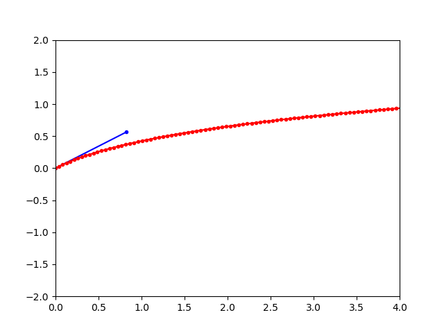
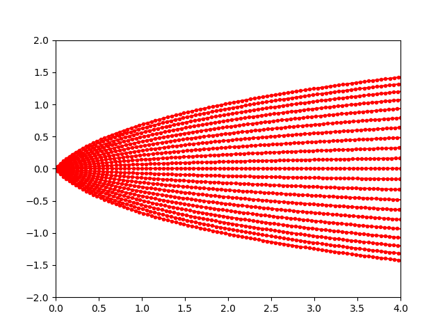
In our iterative approach, instead of generating a long light ray, we generate many connected short light rays to estimate the path of the curved ray. For the 2D implementation, we modeled the ior of the space to be 1+x, so that the ior increases along the path that the light travels. At the first step of the iteration, we generated a very short ray with the initial direction (blue line), and then calculated the direction of the next ray by using snell’s law, and setting the origin of the next ray to be where our current ray ends. We repeated this a couple hundred times to get the approximated path. In the image on the left, the blue ray represents the original direction, and the dotted red line is the actual (approximated) path the light follows. The image on the right shows the estimated path for various rays cast from the origin with directions between -1 and 1 radians.

In the coordinate transformation approach, we can exploit existing linear pathtracing code to trace nonlinear rays through use of a "ray-linearizing" coordinate transformation. Such a coordinate transformation re-expresses nonlinear rays in a new set of coordinates in which light rays must travel linearly. By applying this coordinate transformation to our scene, we can use linear raytracing code to trace nonlinear rays, switching between real and transformed space as needed.

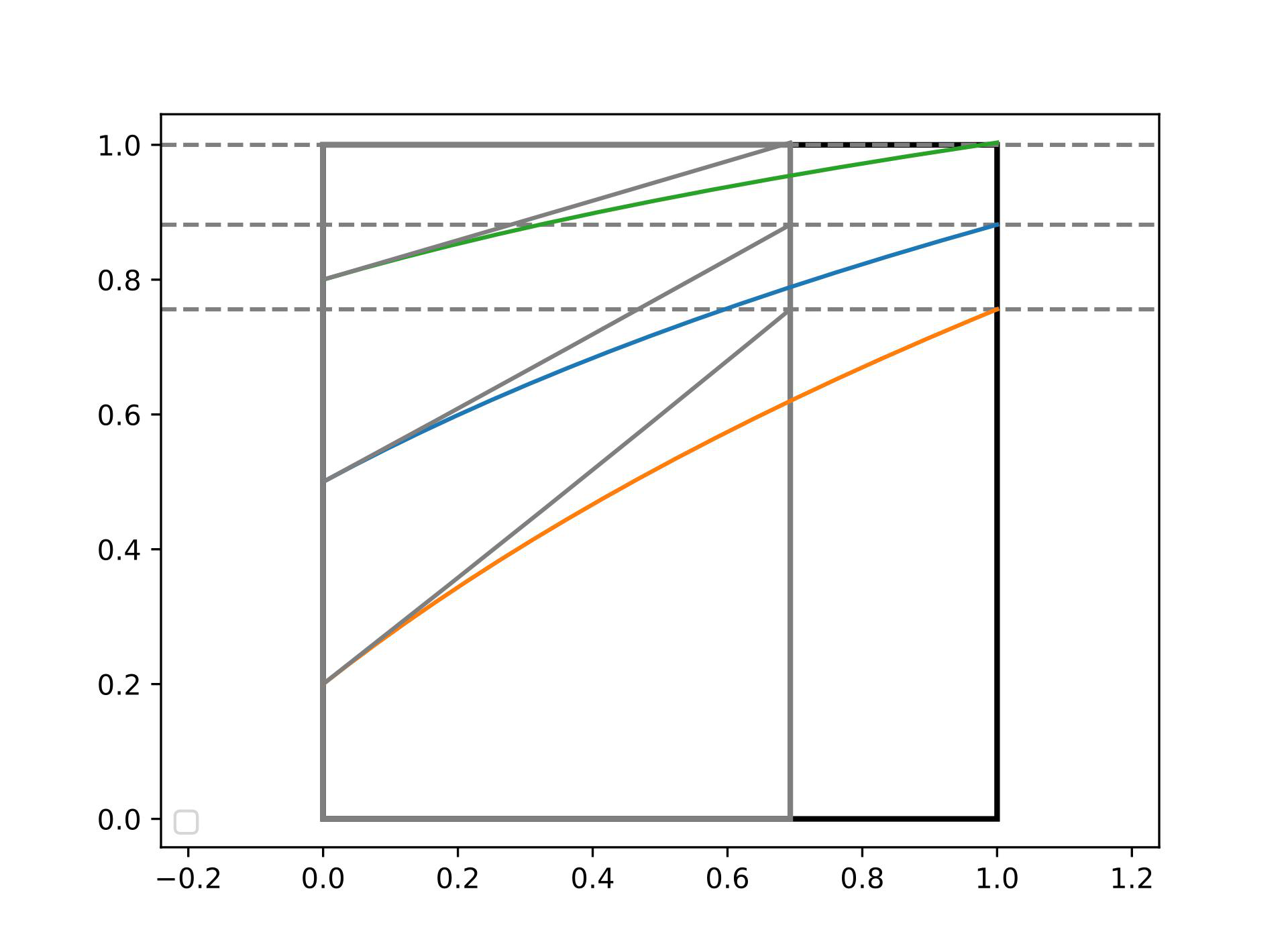
The above figure shows how the coordinate transformation method works in 2D. Colored curves denote iteratively calculated ray trajectories through a $1\times 1$ box (black outline in figure) in a medium with an index of refraction $n = 1+x$. When the coordinate transformtion $x\rightarrow x' = {\rm log}(1+x)$ is applied, these curved rays become straight in transformed space (the grey diagonal lines). By applying this same coordinate transformation to the boundary of the box (grey rectangle), we can use linear ray tracing to find the exit point of our rays in transformed space (dashed grey lines). By appying the inverse transformation $x' \rightarrow x = e^{x'} - 1$, we can determine the ray exit point in real space. From there, we can continue raytracing as normal.

Overall, these usefule results proved that both methods of implementing curved rays could be feasible, and so we decided to use both methods to implement and 3D nonlinear path tracer and then compare their performance.

Scene Creation

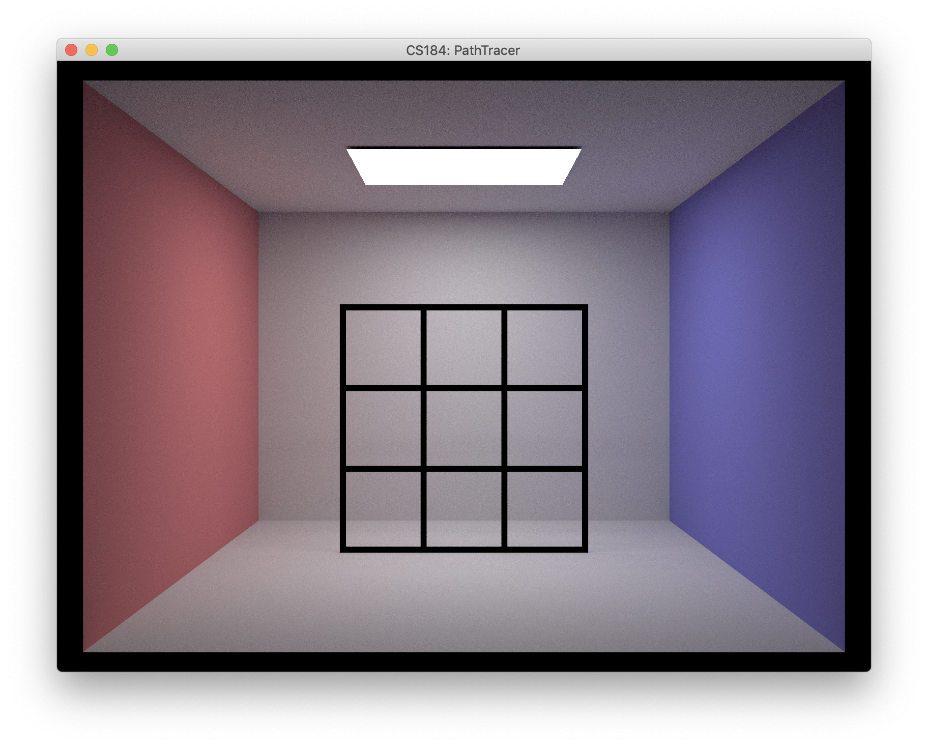
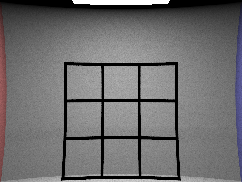
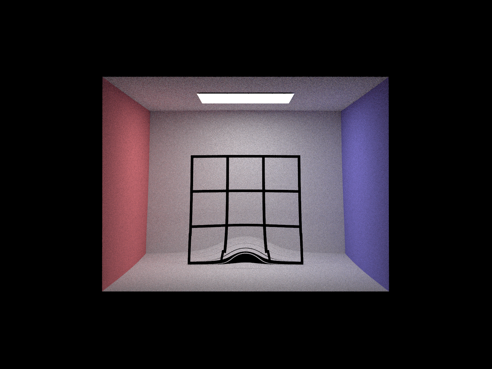
In order to properly visualize the effects of a 3D path tracer, we needed to create a simple 3D scene with a useful structure and reasonably predictable behavior. Not only would this help to easily see the effects of cruved light rays, but it would also help us debug our code if the end result seemed not quite right. We decided that a simple, well-light black grid placed a medium distance from the camera would best fit our needs, so we editted one of the cornel box scenes provided for project 3 by keeping the box mesh and ceiling light but replacing the meshes inside the box with a medium-sized 9x9 with the lines made from simple meshes. This test scene is shown below.

3D Path Tracer: Iterative Approach

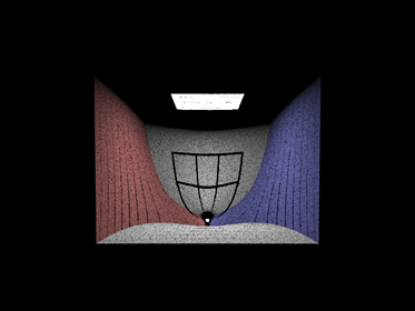
For this method, we built upon the project 3 code by taking the rays generated by the camera and used those rays to approximate the path like in our 2D implementation. In this implementation however, at each iteration, we tested whether or not the ray intersected with the scene. If it did, we returned the estimated radiance. If it didn’t, we calculated the next ray and moved onto the next iteration. We modeled the space to have an ior of 1-z (since the camera faces the negative z axis). The result is below. The reason the image is so zoomed in is because rays generated at the edge of the camera that would normally not intersect with the scene now bend inwards and intersects with objects in the scene.

After we had a more solid understanding of the code structure, we were able to do other cool things like generating a black hole. In this scenario, to calculate the next ray in the iteration, we calculated the pull of the black hole by calculating the vector found by subtracting ray’s origin from the black hole’s origin. We calculated the distance r between the two origins, and then set the magnitude of the pull to be 1/(kr)^2 where k is some constant used to vary the strength of the black hole. This function was a simplified version of the gravitational force equation: GMm/r^2. We added the pull to the previous’ rays direction to calculate the next rays direction, repeated these steps at each iteration until a intersection was detected, and ended up with some really nice results.

3D Path Tracer: Transfomation Approach

Our 2D transfprmation method is easily extended to 3D; we accomplish this by modifying the project 3-2 pathtracing code, with the primary goal of rendering simple gemoetric objects of inhomogenous refractive index. Our primary modification is the introduction of a secondary bounding volume hierarchy (BVH) structure, obtained by applying the ray-linearizing coordinate transformation to the original BVH. We also added in methods for moving points in real space into transformed space, and vice versa. Finally, we implemented methods for moving instantaneous ray directions between real and transformed space. These methods allow us to determine the entering and exiting directions of rays passing through the boundary between the inhomogenous medium and surrounding air, in both real and transformed space. Ray direction transformations are calculated by applying the coordinate transformation (or its inverse) to a pair of closely spaced neighbor points on the ray trajectory, then converting the pair of tranformed points into a unit vector.

The above modifications allow us to render any object whose linearizing transformation is known. The algorithm is as follows:

1. Apply the linearizing transformation to the BVH. Call this BVH2.
2. Given an origin (initially the camera) and direction in real space, cast a ray into the scene and find the nearest ray-scene intersection by testing against the BVH.
3. At the intersection, determine if the ray is about to enter an object with variable IOR. If not, continue pathtracing as normal until either the radiance of the ray is determined (in which case we return) or the ray hits an intersection where it is about to enter the variable IOR medium.
4. Use Snell's law to determine the initial direction the ray will have in the medium, in real space. Convert this initial ray direction to the equivalent direction in transformed space.
5. Using the ray intersection point and direction in transformed space, cast out a new ray, this time testing for intersections against the transformed BVH2
6. Upon finding an intersection, determine if the ray is about to exit the medium. If continue raytracing in transformed space. Otherwise, use Snell's law to determine the exit direction of the ray in transformed space, then convert to an exit direction in real space.
7. Go back to 2.

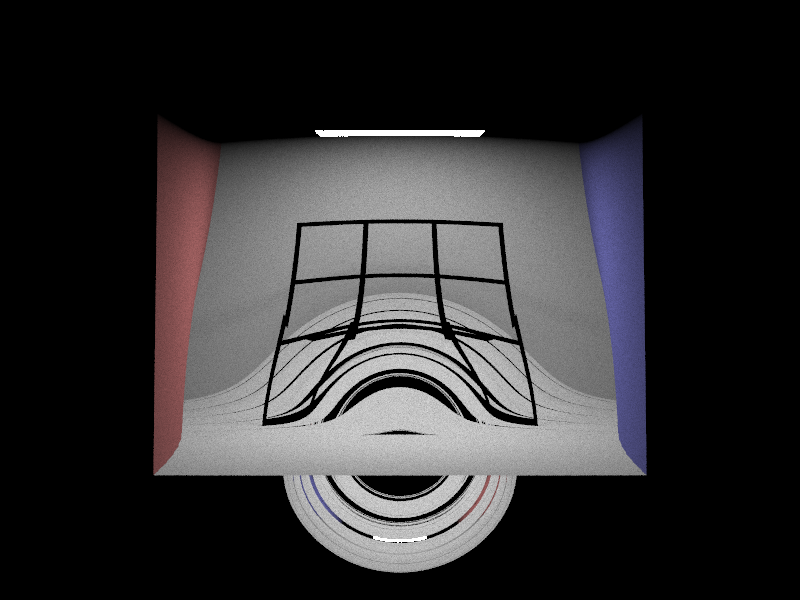
Results of our algorithm are shown below, where we have rendered in our test scene a cube with $n = 4-z$, where $z=0$ at the cube front and increases along the view into the cube. The image is rendered at 128 samples per pixel and 4 samples per light. Note the warped and minified grid image in the cube, as expected according to Snell's law.

Comparison

The transformation approach is relatively fast due to its ability to convert nonlinear raytracing problems into linear ones. However, its use is constrained to scenarios where a ray-linearizing transformation can be found. These transformations can be hard to derive, and most involve solving a differential equation. Even the simple 2D case where $n=1+x$ involves solving the differential equation $$ \dfrac{dy}{dx} = \dfrac{1}{\sqrt{(1+x)^2/a^2 -1}} $$ where $a$ is a constant determined by the entrance angle and IOR of the surrounding medium. This differential equation can be solved approximately in the paraxial limit, yielding the approximate ray trajectory solution $y \propto \log (1+x)$, from which we derived the linearizing transformation $x\rightarrow \log(1+x)$.

Thus, in scenarios where no ray-linearizing transformation is available (most scenarios, we believe, including black holes), the iterative pathtracing method is more applicable. However, in scenarios where the the linearizing transformation is known, the transformation method provides a fast alternative. Such scenarios may become more important in the future, via the growing field of transformation optics (TO). TO relates coordinate transformations to the physical permittivity and permeability distributions a material would need in order to effect such a coordinate transformation in the paths of light rays within the material. Such materials are easily rendered using our transformation pathtracing method since the linearizing transformation will already be known.

Custom Scenes

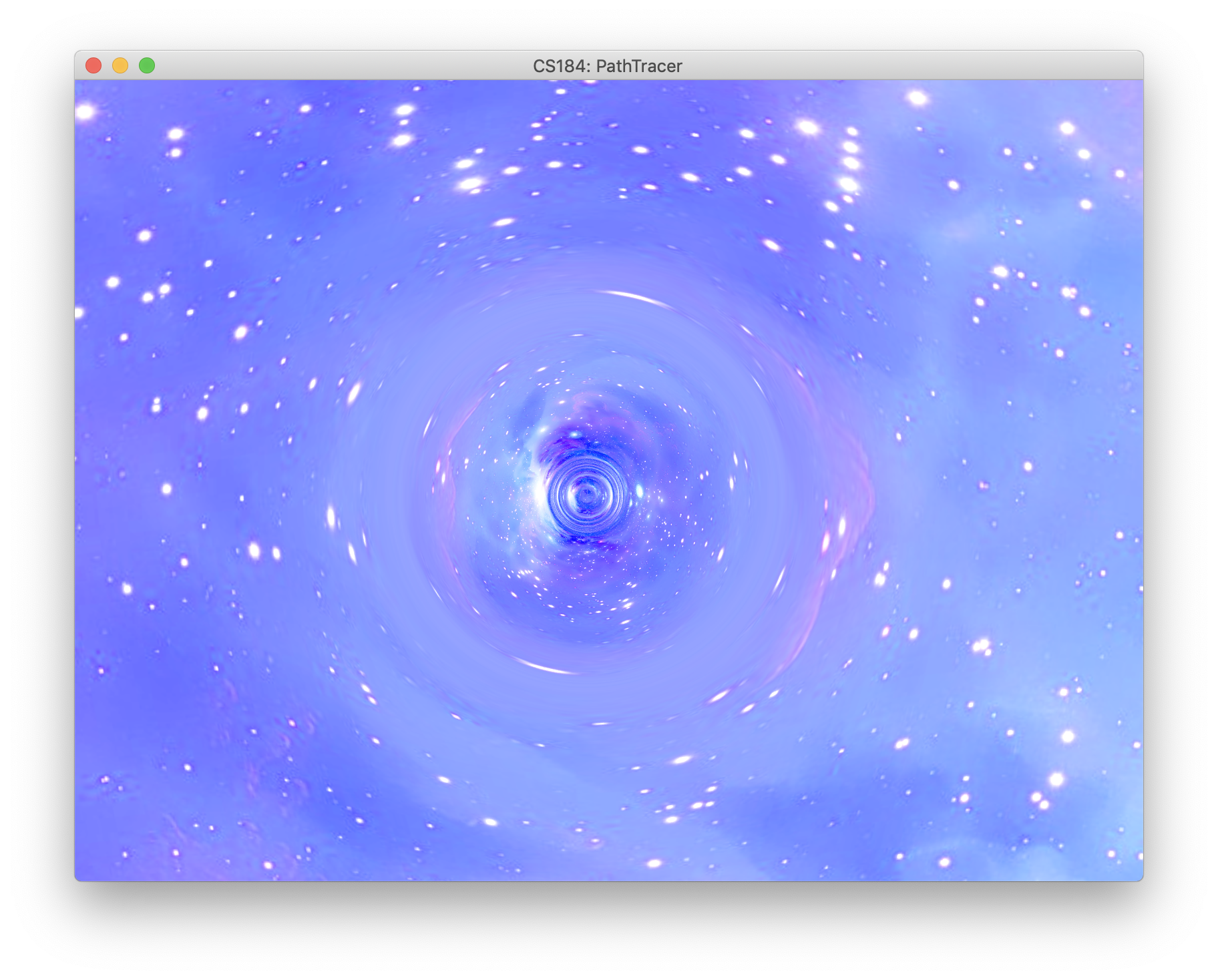
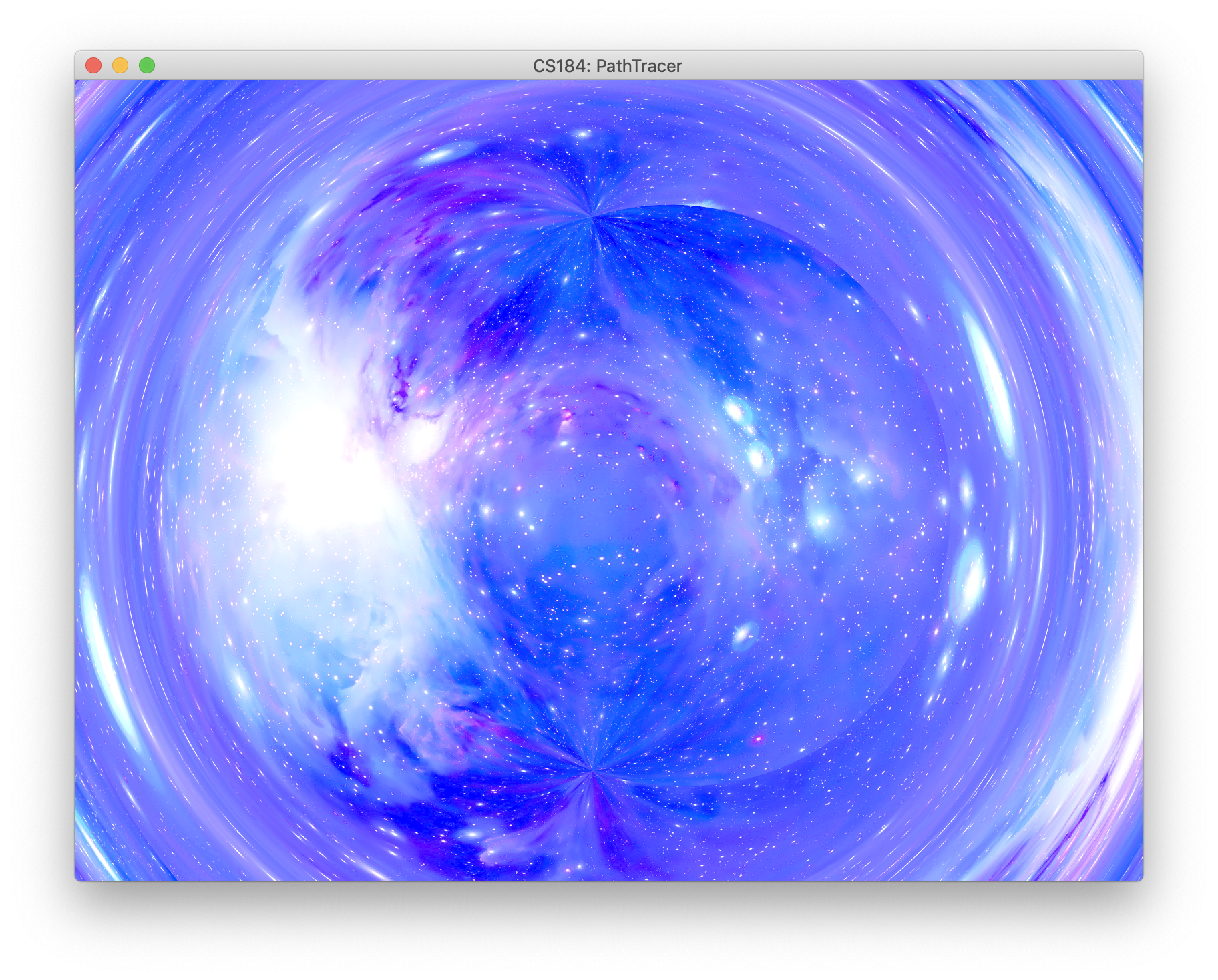
In order to further expand the posibilites for our nonlinear path tracer, we integrated it with project 3-2 so that it could work with more types of surfaces and include environment map support, which is something we were particularly interested in applying the nonlinear pathracing to. In order to get the iterative method working with environment maps, we added the case that when the iteration finishes and the final light ray has still not intersected with anything, then the radiance of this sample is gotten by sampling the environment map (if on exists) in the direction of the final ray. We rendered an empty scene with an added black hole at the origin and a space-themed texture map that included a nebula and some stars. The results below, show the very cool and interesting effects of the curved light rays applied to a environment map. Notice that background distorts more towards the center of the image where the black hole is located. The right image shows a more zoomed-in view focused on the center of the black hole. Note that due to the details of implementation no event horizon exists, and the black hole can be considered "infitesimally small", although the effects of the curved ligh rays are still clearly present.

We also can change the gravity around the origin of the blach hole, which effects how much light is effected by its presence. Below we see some interesting images due to changing this paramter. The left shows the original black hole image of the test scene, and the middle image is what results when decreasing its effect by around 90%. We also fully inverted the effects of the black hole on the light rays by making them be repeled from the center rather than be pulled towards it. The results is shown on the right image.

Problems and Reflections

One of the biggest challenges of the project was adding functionalities to our project 3 pathtracer. We didn't have a complete understanding of the code structure, and that made modifying the code to suit our needs difficult. To deal with this, we traced the code from the ray generation area to the intersection area, and found the methods we needed to modify to meet our goals.

Contributions

William He: Iterative Method

Jonathan Lin: Transformative Method

Ryan Pottle: Test Scene Creation, Environment Map Integration, Video Recordings

References

Below are some resources we used to learn about nonlinear ray tracing and related ideas, as well as the different ways to imnplement it.

https://physics.stackexchange.com/questions/122599/ray-tracing-in-a-inhomogeneous-media

Ray tracing in inhomogeneous, but optically isotropic media. Talks about the “eikonal” equation.

https://arxiv.org/pdf/0805.4778.pdf

One of the first papers written about transformation optics, where you model the curvature of light rays/deformation of waves as a coordinate transformation.

https://graphics.stanford.edu/courses/cs348b-competition/cs348b-05/mirage/index.html

An example implementation of a simple nonlinear ray tracer. Index of refraction profile is assumed to be linear. Different numerical methods for iteratively calculating ray trajectories are presented.